Real power saves you but post-hoc power tricks you


TL;DR
-
Power analysis is your experiment’s safety net in fixed-horizon frequentist test
-
Without it, non-significant results mean nothing: You can’t tell if there’s no effect or just not enough data.
-
Without it, significant results can mislead: Effect sizes may be exaggerated by chance.
-
Post-hoc power adds no value: It can’t rescue a poorly planned experiment.
-
Do it right: Define a meaningful MDE, plan for at least 80% power, and stick to your sample size plan.
Power analysis is important and what will happen when you skip it
Every textbook on fixed-horizon frequentist testing emphasizes the importance of doing a power analysis when designing experiments. That’s because power analysis tells you how much data you need to make sure your results are reliable for decision making.
- Example Checklist
To show why “planning for enough data” matters so much in this type of test, we run experiments without power analysis and see what happens.
Suppose we made the checkout button more visible (at the cost of some fun cats) and expected it to boost conversion. But instead of using power analysis to plan the sample size and run time, we just picked a timeline based on convenience or stakeholder pressure.

Image source: Optimizely
Scenario 1: Without power analysis, a non-significant experiment can be confusing.
Does the non-significant result mean our expected positive effect in the hypothesis is unlikely to exist? We don’t know. The crowded checkout page may not bother cat lovers, resulting in no impact from simplifying the checkout button. However, a more likely scenario is that we simply don’t have enough data to spot any impact.
Let’s set the cat checkout page with a conversion rate of 0.2 and the no-cat checkout page with a conversion rate of 0.25. So, we know there is a 25% lift in conversion rate lift (a quite large effect we don’t want to miss!).
We did not do a power analysis, so we’ll simulate data for different sample sizes. For each size, we generate 1000 different datasets to reflect the natural variation in sampling and run the hypothesis test on each dataset.
To show the chance of successfully detecting the effect at each sample size, we’ll record the percentage of tests at each sample size that detect a 25% lift and reject the null hypothesis.
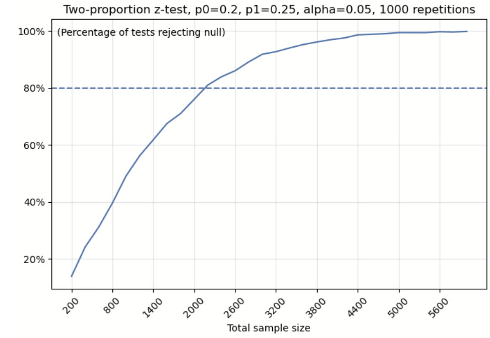
Image source: Optimizely
The line chart above illustrates that as the sample size grows, the chances of rejecting the null hypothesis also increase, which boosts our ability to spot that 25% lift. However, when our sample size drops below 2000, our chance of detecting the 25% lift is below 80% and we are more likely to miss the effect.
Some people might think, okay, I get that if we skip power analysis and get a non-significant result, we can’t tell if there’s truly no effect or just not enough data. But take a look at the graph. Even with just 1,400 samples, we still have over a 60% chance of detecting a lift. That’s actually pretty encouraging. So if our sample size isn’t too small, it might feel okay to run the experiment without doing power analysis first.
But here’s the catch: if we skip power analysis to secure a big enough sample size and still get a significant result, we can’t fully trust it. The estimated effect might be off or exaggerated too much.
Scenario 2: Without power analysis, a significant experiment can still be misleading.
Let’s look again at the same simulation from Scenario 1. This time, we focus on how often significant results show the wrong effect—specifically, when the estimated effect is negative, even though we know the true effect is positive. We calculate the percentage of significant results returned negative effects at different sample sizes.
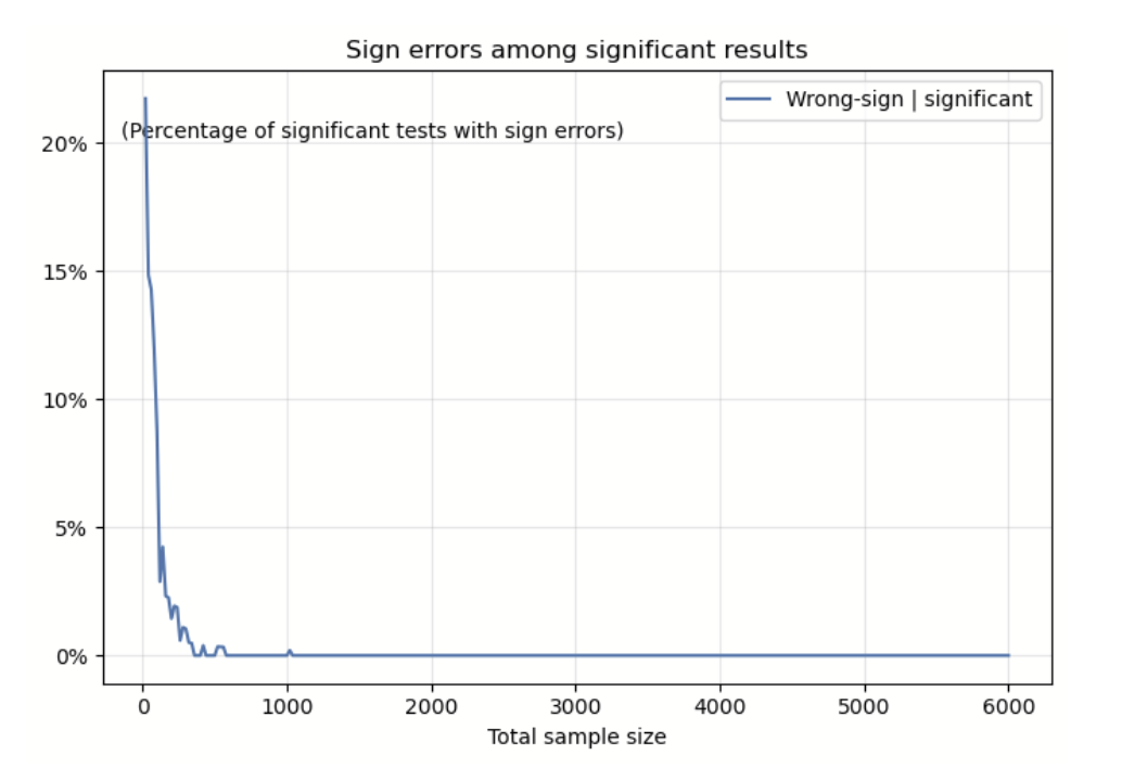
Image source: Optimizely
Two things stand out in the chart above:
-
It's possible to get a significant result where the estimated effect is completely wrong.
-
These errors become less common as the sample size increases. (However, in our simulated data, even with 1,000 samples, there’s still a small chance of getting the wrong direction.)
What if our significant results point in the right direction?
We looked at that too. We calculated the average estimated effect among all significant results that correctly showed a positive effect.
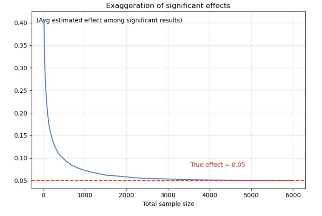
Image source: Optimizely
The chart above highlights two key points:
-
Even when the estimated effect has the correct sign, it can be much larger than the true effect.
-
This exaggeration gets smaller as the sample size increases.
The sign and exaggeration errors we looked at come from a framework by Gelman & Carlin (2014), known as Type S (Sign) and Type M (Magnitude) errors. Our calculations aren't exact replications of their method, but they capture the core idea: significant results can sometimes point in the wrong direction (Type S error) or exaggerate the size of the effect (Type M error), especially when we don’t have enough data.
By now, it’s clear why having enough data is key to getting reliable and useful results.
How does power analysis help with that?
Take another look at the first line chart. We usually consider a sample size “enough” if it gives us at least an 80% chance of detecting a true effect. This is what we mean by 80% power. In our simulation, that corresponds to about 2,500 samples. So, if you run an experiment with 80% power and get a non-significant result, you know that the effect you expected in your alternative hypothesis probably isn’t there.
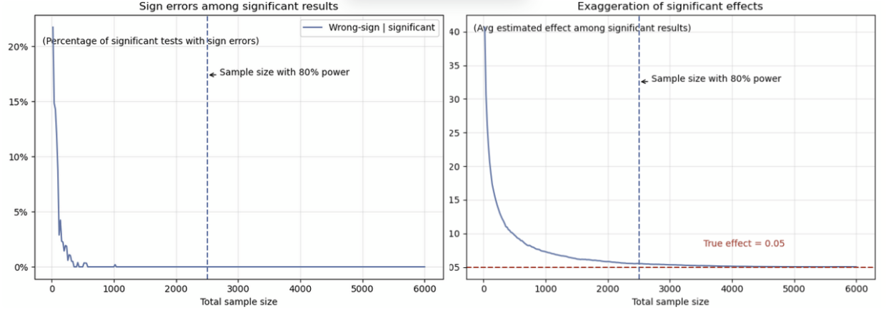
Image source: Optimizely
On the other hand, if you get a significant result with 2,500 samples (i.e., an experiment with 80% power), the chances of it being wrong or overly exaggerated are very low. That means you can trust the result to guide your decisions.
In short, power analysis helps you plan for enough data to make both non-significant and significant results trustworthy.
Now, for whatever reason, we didn’t do a power analysis before starting an experiment. Can we do it afterward and still learn something useful? Unfortunately, no.
The limited usefulness of the post-hoc power analysis
To understand the problems of post-hoc power analyses, we first need to grasp how power is defined in frequentist statistics.
The definition of power
The “power” is the probability of correctly rejecting the null hypothesis. Like other concepts in frequentist statistics, such as the false positive error, the power is defined across a series of repeated experiments under identical conditions, which can confuse many applied users.
To understand the concept, let us reuse the checkout button experiment mentioned above. The figure below defines the power for this hypothetical experiment.
In practice, we would conduct one experiment on the checkout button and compute the associated p-value (i.e., Experiment 1 in the figure). However, the power is derived from not only this experiment (i.e., Experiment 1) but also from potential experiments we could conduct (i.e., experiments 2, 3, …, M). This is what we mean by “the power is defined across a series of repeated experiments under identical conditions”. Since we do not observe the other potential experiments, we actually do not know the “real” power in an empirical setting; This is also why, to illustrate the behaviour of the power, we typically rely on simulation studies (like the ones above).
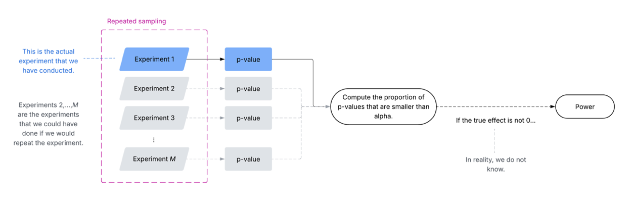
Image source: Optimizely
In an empirical setting, we don’t know the true effect. So, when planning an experiment, we plug in the minimum detectable effect (MDE)—the smallest effect we care about—to estimate the sample size.
This ties directly into how hypothesis testing works. The test only tells us whether we can reject the null hypothesis. It doesn't confirm whether the effect we put in the alternative hypothesis (like the MDE) is the true effect, because we don’t know what the true effect is.
If we reject the null with enough power, it means we found strong evidence that a real effect exists. However, we should also check how large that effect is. If the observed effect is smaller than the MDE, it may be statistically significant but not practically meaningful — in other words, the change is real but might not be large enough to justify action. If we don’t reject the null, it means either there’s truly no effect, or the current sample size is not large enough to detect the effect.
Can we instead use the effect we observe from the experiment to calculate power afterward (a post-hoc analysis)? No, we can’t. The estimated power can be noisy and using it this way can give a very misleading picture of power.
The post-hoc power
Let’s reuse the checkout button experiment example. We collected 100 visitors for the control group and 100 for the treatment group. The conversion rate for the control group is 0.90, while the treatment group is 0.94. The observed (nonstandardized) effect size (i.e., difference in means) is 0.04, with a standard error of approximately 0.0383. Given the critical value of 1.96 (two-sided test, alpha=0.05), the p-value is 0.396, and the 95% confidence interval is (-0.0351, 0.1151) based on the Wald test for the mean difference. This confidence interval may be regarded as the plausible range of the true effect given the data and information. If we plug in each value in this interval as the true effect, then the power can be estimated based on the formula (Wasserman 2012):

Where the delta is the plug-in value for the effect. The table below shows the estimated power based on several possible values of the true effect.
| Possible values of the true effect | Estimated power |
| 0.1151 | 85% |
| 0.107 | 80% |
| 0.04 | 18% |
| 0.001 | 5% |
| -0.0351 | 15% |
Thus, depending on the possible values for the true effect suggested by the confidence interval, we estimate that the power ranges from 5% to 85%, and this range is too large to be of any practical use.
A post-hoc power analysis does not offer extra insights
We repeat the point that has been made previously:
From the statistics perspective, whenever a result is not statistically significant, either the true effect is zero, or the sample size is not enough to detect the effect (and therefore the study is under-powered). We cannot determine which is the case.
This statement does not require a post-hoc analysis, and a post-hoc analysis does not offer extra insights beyond the statement. As shown in the table above, the estimated power is mostly below 80% for the range (-0.0351, 0.1151), which is unsurprising since the result is not significant. The real problem, however, is that we do not know whether the true effect is zero or not, and this question cannot be addressed by a post-hoc analysis.
Post-hoc power as a bias detection tool
We have established that post-hoc power is not useful for evaluating a single experiment. However, it can help assess the credibility of multiple studies in an academic paper. This topic exceeds this blog's scope; interested readers are advised to read Schimmack (2012) and Aberson (2019, pp.15-16).
Best practices for power analysis in fixed-horizon frequentist tests
Power analysis isn’t just a box to check—it’s the foundation of running trustworthy experiments. To make your results both believable and actionable, keep these principles in mind:
-
Define and defend your MDE: Don’t pick a “detectable effect” out of thin air. Think through what size of improvement is practically meaningful and justify it. But remember, MDE isn’t the true effect but just the effect you care.
-
Plan your sample size upfront: Base it on at least 80% power for your chosen MDE, and pay close attention to the assumptions behind your calculation method (we will discuss it in details in another blog post).
-
Commit to the plan: Once the experiment starts, strictly stick with the predetermined sample size based on power analysis.
-
Power analysis helps beyond fixed-horizon frequentist tests: Not all studies need power analysis from a statistical standpoint. For example, Bayesian approaches or our sequential tests don’t rely on fixed sample sizes in the same way. However, power analysis can still be useful in these settings to help guide your experiment design
Thoughtful power analysis transforms your test from a gamble into a reliable decision-making tool. Skip it, and your A/B test is no better than a coin flip. Do it wrong, and it offers false comfort instead of real insight.
References
Aberson, C. L. (2019). Applied power analysis for the behavioral sciences. Routledge.
Gelman, A., & Carlin, J. (2014). Beyond power calculations: Assessing type S (sign) and type M (magnitude) errors. Perspectives on psychological science, 9(6), 641-651.
Schimmack, U. (2012). The ironic effect of significant results on the credibility of multiple-study articles. Psychological methods, 17(4), 551.
Wasserman, L. (2013). All of statistics: a concise course in statistical inference. Springer Science & Business Media.

Qian Zhang is a Senior Statistician at Optimizely specializing in experimentation, causal inference, and product analytics for large-scale digital platforms. Prior...

- Last modified:2026-02-13 00:38:45