Sample size calculations unpacked: Origins, hidden assumptions, and trade-offs


TL;DR
- Sample size calculations in experiments are all about balancing error rates (Type I & II).
- Use sample size calculation formulas that match your test design and assumptions (like equal variances or group sizes).
- You can shrink the sample size by choosing metrics with lower variance or accepting a larger MDE, but always ensure your choices match your business reality.
- At Optimizely, sample size estimation is tailored to the specific test and metric, using the delta method for relative lift.
If you’ve ever tried planning sample size for an experiment, you know the internet is full of formulas. But not all formulas are created equal. Each comes with assumptions that may or may not match your test and data reality. And beyond those basics, there are a few practical nuances that can make or break your experiment’s success.
The origin of sample size estimation (Error control for hypothesis test) enhancement_commerce-analytics
When you run a hypothesis test in an experiment, you end up making one of two decisions: either reject the null hypothesis H0 or don’t reject it. But this decision can be wrong since it’s based on just one sample from all the data you could have. In Frequentist hypothesis testing, we call these mistakes Type I or Type II errors, as shown in the table below.
| Reject H0 | Not reject H0 | |
| H0 True | ✕ Type I Error | ✓ |
| H1 True | ✓ | ✕ Type II Error |
Usually, we evaluate a hypothesis test by its probabilities of making Type I (α) and Type II Errors (β). A good test or experiment tries to keep these probabilities low enough so we can trust the results and make good decisions based on the experiment.
Any test has a rule to decide when to reject H0. Usually, this rule checks if the observed effects fall inside a “rejection region” R. If they do, we reject H0; if not, we don’t. If we define the probability of rejecting H0 as Pr(observed effects ∈ R), this probability means different things depending on whether H0 or H1 is true.
- When H0 is true, Pr(observed effects ∈ R|H0 is true) = Pr(reject H0|H0 is true) = Type I Error probability
- When H1 is true, Pr(observed effects ∈ R|H1 is true) = Pr(reject H0|H1 is true) = 1-Pr(not reject H0|H1 is true) = 1- Type II Error probability
Put formally, we can define the function based on θ (Casella & Berger, 2002):

Statisticians call this the “power function” because 1 - Type II Error probability is the probability of correctly rejecting H0 when H1 is true— what we call the test's power. This single function combines information about a test’s probability of making both Type I and Type II Errors and thus is used to evaluate and compare different tests.
Here's an example: the graph below shows how the power functions of two tests change depending on the true effect θ on the x-axis. Let's say our hypothesis is H0: θ ≤ 0.5 versus H1: θ > 0.5. The function β1(θ) tells us that test 1 has a low probability of a Type I Error when θ ≤ 0.5, but it has a high probability of a Type II Error (i.e., low power) when θ > 0.5. In contrast, β2(θ) shows that test 2 has a higher probability of a Type I Error when θ ≤ 0.5, but a lower probability of a Type II Error (i.e., higher power) when θ > 0.5. If you have to pick between these 2 tests, you need to decide which kind of error pattern—β1(θ) or β2(θ)—you find more acceptable.

Now, you might wonder what shapes the curve of β(θ) in the graph. It depends on:
-
What type of test you pick
-
After picking the test type, how you set it up, such as the sample size and/or Type I/II Error threshold in the test.
The Wald Test dominates fixed-horizon Frequentist tests in industry A/B testing because it’s computationally simple and highly accurate at large scale (for detailed theoretical foundations of Wald type tests, see Wu& Ding ,2021, Ding, 2024, Imbens & Rubin, 2015).
For two-sided Wald Test, the power function is approximately:
 Then,
Then,
 This last equation shows how people come up with different formulas for sample size (for more examples of sample size estimation based on power functions, see e.g., Chow et al., 2017, Stuart et al., 2004, Casella & Berger, 2002, Davison, 2003, Cox & Hinkley, 1979). Specifically, changes depending on the assumptions you make.
For example, when you're testing the absolute mean difference between two groups, a treatment group and a control group (which is the most common setup in A/B testing), you might see different sample size formulas. It depends on assumptions like the ones in the table below.
| Variance assumption | Sample size assumption | SE0 | Per-group sample size formula |
| Equal variance | equal sample size / unequal sample size |  |
|
| Unequal variance | equal sample size / unequal sample size |  |
 |
-
 is determined by your hypothesis. Specifically, it is the minimum detectable effect (MDE) you are interested in.
 -
 have corresponding values once you decide on values of α and β
A different lens: Alternative paths that lead to more sample size formulas
Belle (2011, pp. 27-29) explained how sample size is calculated from a slightly different angle.
Suppose we are going to run a randomized experiment with a control group and a treatment group for testing a new feature. Formally, we specify the hypotheses as follows:
H0 (null hypothesis): No difference between control and treatment groups.
H1 (alternative hypothesis): A difference exists between control and treatment groups.
Further, we assume the false positive rate is alpha (typically 1%, 5%, or 10%), the false negative rate is beta (usually 20%), and the mean difference between the two groups is delta (e.g., minimal detectable effect; MDE). Figure 1 shows the sampling distributions under the null and alternative hypotheses. Under typical circumstances, the sampling distributions are approximately normal distributions when the sample size is large enough.
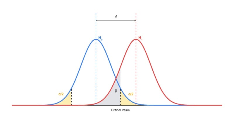 Image: Sampling distributions
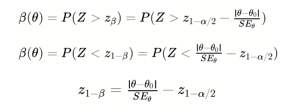
If the null hypothesis is true, then we have the following fact: Given alpha, the critical value (i.e., the boundary for not rejecting the null) must be equal to:
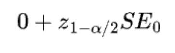 Where
Where
 is the z-score at 100(1-alpha/2)th percentile and SE0 is the standard error under the null.
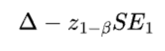
If the alternative hypothesis is true, then we have the following fact: Given beta, the critical value (i.e., the boundary for rejecting the null) must be equal to:
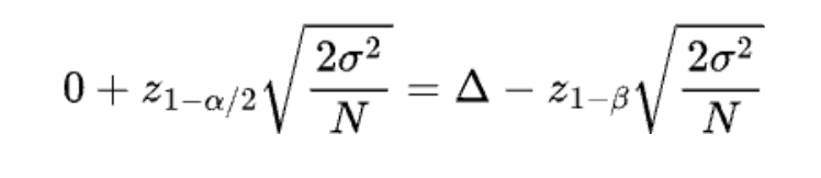
 Because the critical value is for defining the boundary for the rejection and the acceptance region, we must have

This is the general formula that underlies sample size estimation. At first glance, it seems unrelated to sample size, but standard errors depend on sample size and other factors. Similarly, you can also get different sample size options using this general formula. For example, for testing the absolute mean difference between a treatment group and a control group, you can come up with different sample size formulas based on assumptions like the ones in the table below.
To keep it simple, we assume a z-test and equal sample sizes n. You can find formulas for unequal sizes by setting![]()
| Variance assumption | SE1 | SE0 | Per-group sample size formula |
| Equal variance |  |
Same as SE1 |  |
| Unequal variance |  |
Same as SE1 |  |
| Unequal variance | |
Different from SE1
|
 |


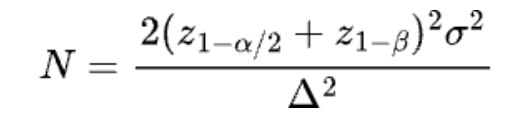
The simple “rule-of-thumb” formula
Most sample size formulas you see for online A/B testing come from the general formulas based on those two frameworks above. For example, let's break down the well-known “rule-of-thumb” sample size formula ![]()
It is often usedin industry for a “quick estimation” of sample size.
Let’s assume:
- The control and treatment groups are generated by normal distributions with the same variance
- Equal traffic split, with each group having a sample size of N.
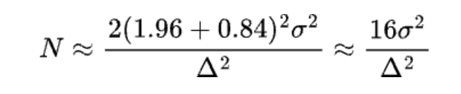
Then general equation above becomes
 We can easily derive the sample size N by solving this equation
 If α=0.05 and β=0.2, then
Best practices for picking a basic formula:
Here are two bottom lines about picking sample size formulas:
- Match the formula to the test: Your sample size should match the statistical test you plan to use. Each test defines its own critical region and standard error, so your sample-size formula should mirror those specifics.
- Know what assumptions you’re buying into: Every formula makes some assumptions to keep things simple such as equal group sizes, equal variances, large-sample normality, constant variance across means, and so on. Always ask: Do these assumptions actually hold in my experiment?
In short:
The right formula is the one that matches your test design and data-generation reality.
At Optimizely, we set up a Wald test (z-test) for our Fixed-horizon Frequentist test. We assume the groups have different sample sizes and variances.Using the power function framework, we pick the sample size formula shown below:

Sample size estimation for relative improvement and sample size reduction
When you want to test relative improvement.
The formulas above help figure out the sample size needed to test the absolute mean difference between two groups. Butin business, people usually like to talk about relative uplift instead.
For example, if the conversion rate is p0 = 0.1 and p1 = 0.15, the absolute difference is p1 - p0 = 0.05, while the relative difference is (p1 - p0) / p0 = 0.5, or 50%.
There are two common ways to estimate the sample size for testing relative differences between groups.
| Method | Description | Binary metrics example |
| Absolute-difference approximation | Translate the relative lift into an absolute difference. Then, use the sample size formula for absolute difference. |
|
| Delta method | Directly use the relative improvement. Use a first-order Taylor expansion to estimate its variance |
|
How much difference are the two methods making in practice?
To compare the two methods, we ran a simulation to check if the sample sizes planned for relative improvement actually reach the power we want in actual tests. The diagram below shows how we did the simulation.
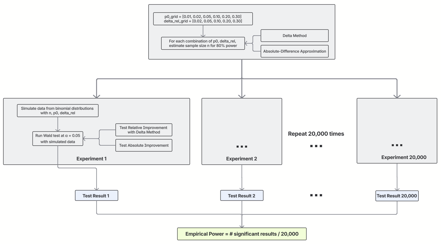 Note that we also varied the actual tests in the simulation. Like with the two ways to estimate sample size, if you want to check for relative improvement, you can turn the relative lift into an absolute difference and test that, or you can use the delta method to test the relative improvement directly. The simulation results are shown below.
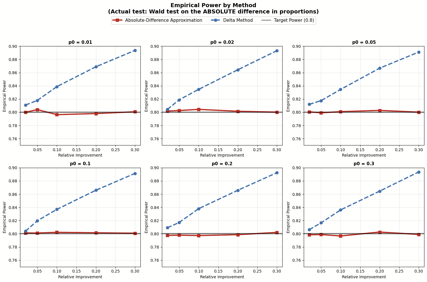 Image: Simulation results testing absolute mean difference
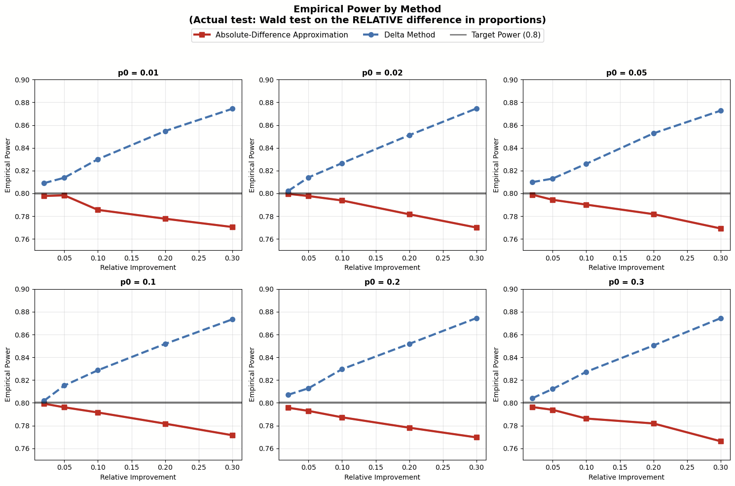 Image: Simulation results testing relative mean difference
The simulation results suggest:
- When testing absolute mean difference, the Absolute-Difference Approximation for planning sample size matchesour goal of 80% power. On the other hand, the Delta Method tends to overestimate the sample sizes needed.
- When testing relative mean difference with the delta method, the Absolute-Difference Approximation usually underestimates the sample sizes because it underestimates the variance. The problem of being underpowered gets worse as the relative improvement grows.
These findings highlight our suggested best practice earlier: make sure your sample size estimation matches the statistical test you plan to use. If you're using an absolute difference test to estimate a relative difference test, go with the Absolute-Difference Approximation for your sample size. But if you run the relative difference test directly using the delta method, then use that method to estimate sample size. (Picking between these two tests for relative improvement is beyond the scope of this post, but just know that the approximation test skips over some uncertainty in the denominator and isn't the best choice in the industry.)
At Optimizely, we use the delta method to test relative improvement, so our sample size estimation also uses the delta method.
What sample size formulas tell about sample size reduction
When people plan sample sizes, they usually want them as small as possible to keep experiments quick. Two importantfactors that influence sample size often get missed in sample size formulas: the minimum detectable effect (MDE) in the denominator and the metric variance in the numerator. These factors can actually help lower the needed sample size. In all formulas, if we fix α at 0.05 and β at 0.2 (80% power), having lower metric variance or/and a bigger MDE means you need a smaller sample size.
This brings up two practical tips:
- Once you’ve identified candidate metrics that your experimental changes can actually move and that the business cares about the most, you can look at historical data to pick the metric with lower variance as the primary metric. (With historical data, you might be able to reduce sample size further by using techniques like CUPED)
- If stakeholders are rushing you, explain that choosing a bigger MDE can help finish the experiment on time. Butthey should know this means there's a higher chance of missing small effects, so they might want to rethink whatthe experiment is for. And whatever MDE you pick must still be realistic — inflating it beyond what’s plausible simply to finish sooner makes the experiment meaningless.
References
Chow, S. C., Shao, J., Wang, H., & Lokhnygina, Y. (2017). Sample size calculations in clinical research. Chapman and Hall/CRC. (pp. 13-15, 77)
Stuart, A., Ord, K. & Arnold, S. (2004). Kendall's advanced theory of statistics, classical inference, and the linear model. John Wiley & Sons. (pp. 190-191)
Casella, G., & Berger, R. (2002). Statistical inference (2ed). Chapman and Hall/CRC. (p. 385)
Davison, A. C. (2003). Statistical models. Cambridge University Press. (p. 334)
Cox, D. R., & Hinkley, D. V. (1979). Theoretical statistics. CRC Press. (pp. 103-104)
Belle, G. van. (2011). Statistical Rules of Thumb. John Wiley & Sons.
Wu, J., & Ding, P. (2021). Randomization tests for weak null hypotheses in randomized experiments. Journal of the American Statistical Association, 116(536), 1898-1913.
Ding, P. (2024). A first course in causal inference. Chapman and Hall/CRC. pp.25-55
Imbens, G. W., & Rubin, D. B. (2015). Causal inference in statistics, social, and biomedical sciences. Cambridge university press. pp.83-112

Qian Zhang is a Senior Statistician at Optimizely specializing in experimentation, causal inference, and product analytics for large-scale digital platforms. Prior...


- Zuletzt geändert: 12.12.2025 06:09:43