
Understand what p-value exactly means and the limitations of p-value-based decisions.
1
P-value thresholds (also called significance/α level) such as 0.05 are valid tools for long-run error control. However, treating them as strict yes-or-no decisions fails when results are close, like p = 0.04 versus p = 0.06. Focusing too much on this decision rule also distracts teams from considering practical significance and learning opportunities from non-significant results.
2
Modern hypothesis testing combines two distinct frameworks; however, this hybrid approach confuses continuous evidence from a single experiment (Fisher’s p-value) with long-run error control across multiple experiments (Neyman–Pearson hypothesis testing). Understanding their historical contexts clarifies p-value interpretation.
💡Best practices:
|
Every day, companies use online experiments to make decisions in a similar way: they run an A/B test, wait for the p-value to drop below a threshold (like 0.05 or 0.1), call it a win, and then ship the winner.
This approach makes sense, and the threshold exists for good reasons. But imagine this: Two analysts run an A/B test on a checkout flow. They gather data for two weeks, run their tests, and check the results. Analyst A gets p = 0.04 and says, "It's statistically significant, let's ship it." Analyst B runs a nearly identical test the next week, sees p = 0.06, and decides to kill the feature — "Not significant, so the variant doesn't work."
Not shipping the p = 0.06 variant is understandable. What's costly is what happens next: the experiment gets archived, the variant gets forgotten, and the team learns nothing from it. The two p-values only differ by 0.02. The data behind them probably tell the same story. Yet one result leads to action, and the other just gets ignored. That silence is where the real loss is. Online testing tools have made A/B testing quicker and cheaper, but they’ve also made it easier to treat non-significant results as a dead end instead of a question worth revisiting.
How the p-value gets used in online testing and where It goes wrong
In most online experimentation setups, the workflow for a fixed-horizon experiment looks roughly like this:
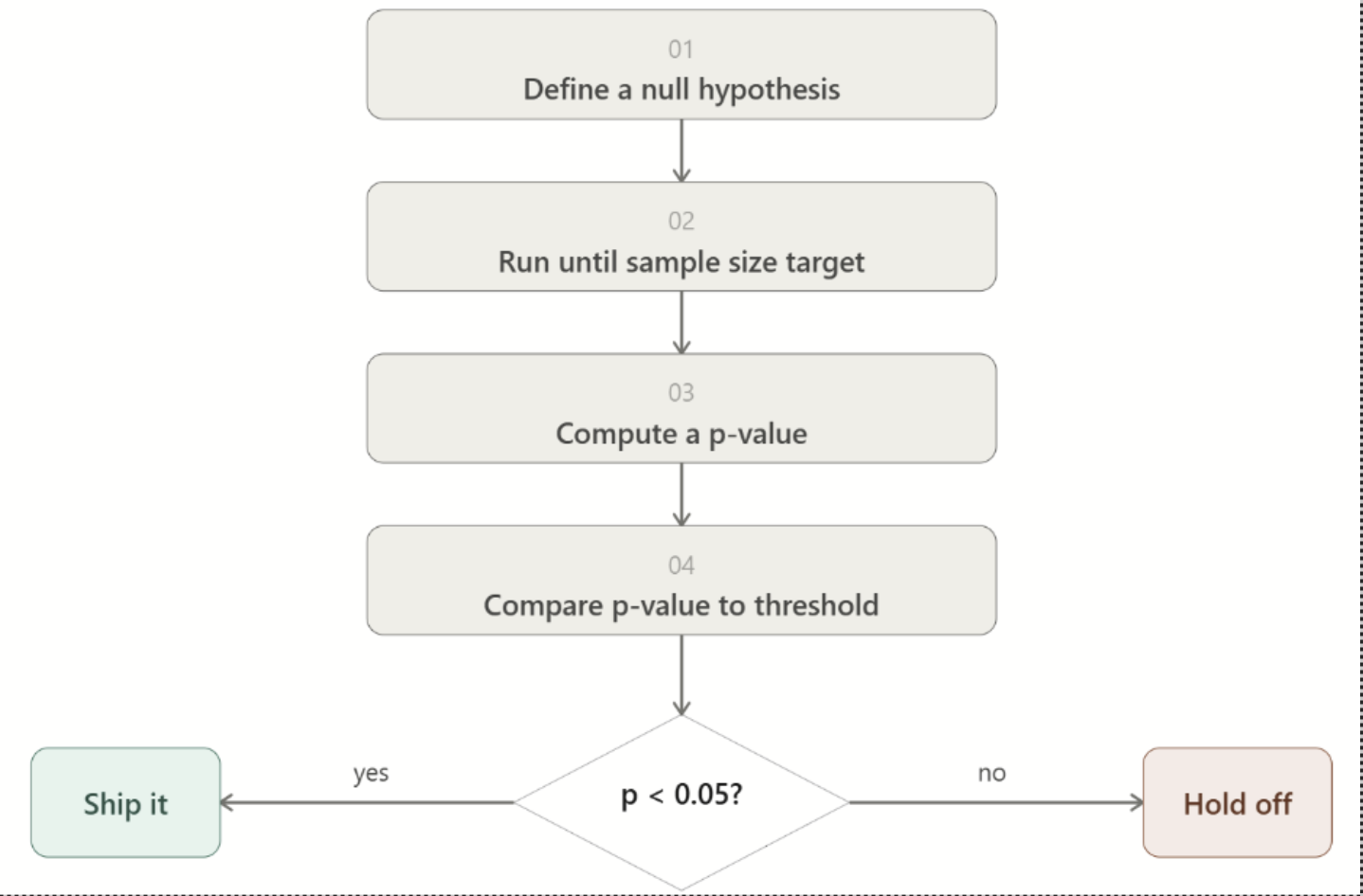
Image source: Optimizely
This workflow isn't wrong in itself, and the threshold is there for a good reason, which we'll explain. But people often misunderstand it, and that confusion leads to real problems in certain cases.
As Greenland et al. (2016) document in their catalogue of 25 common misinterpretations, each of these misconceptions dominate applied practice. Let's go through the ones that matter most in an A/B testing context.
Misinterpretation #1: "P = 0.03 means there's a 3% chance this result happens by chance."
This is the single most dangerous misconception in industry A/B testing. The p-value is not the probability that your result occurred by chance, and it is not the probability that the null hypothesis is true.
The p-value is computed assuming the null hypothesis is true. It represents the probability of observing data this extreme or more so if no real effect exists. Practically, a p-value of 0.03 indicates your data would be unusual if H₀ were true. It says nothing about how probable H₀ is. Those are very different questions.
Misinterpretation #2: "P = 0.04 and P = 0.06 are fundamentally different results."
When results land cleanly on one side or the other (say, p = 0.001 or p = 0.40), the threshold does its job well. The problem arises at the edges. Gelman and Stern (2006) noted that the difference between "significant" and "not significant" is not statistically significant. A p-value of 0.04 and one of 0.06 reflect similar evidence, especially when accounting for measurement error, novelty effects, and test population drift. Treating them as fundamentally different outcomes misrepresents the data reality.
This is critical in online testing, where experiments with p = 0.06 are shelved and those with p = 0.04 are shipped. A coin-flip difference is treated as categorical truth. That'swhere the threshold stops being a useful heuristic and starts being a broken compass.
Misinterpretation #3: "Statistical significance means practical significance."
A feature that increases click-through rate by 0.01 percentage points can be statistically significant with a large enough sample. However, that lift may be meaningless for your business. Statistical significance reflects how surprising the data are, not the effect's size or practical importance. Estimating effect size and its uncertainty is more important for business decisions than the significance label alone.
The source of the confusion: A tale of two frameworks
To understand why p-values often get misused in A/B testing, you should know they come from two different people with very different goals. Nowadays, their ideas got mixed together in a way that neither of them would have agreed with.
1
Fisher's p-value: Evidence, not decision
Ronald Fisher came up with the p-value to measure evidence, not to make decisions. You start with a null hypothesis (there's no difference between variant A and B), gather data, and then figure out how surprising your results would be if the null were true. A smaller p-value means your data looks more unusual if the null hypothesis is correct. Fisher thought of the p-value as just one piece of info a thoughtful scientist weighs alongside prior research, domain knowledge, and context. He even said no one should blindly use a fixed cutoff like 0.05 for every experiment (Fisher, 1956, as cited in Greenland et al., 2016). The famous 0.05 cutoff was just a simple rule of thumb from an era when computing exact p-values by hand was tedious.
Two things are important to note: Fisher's framework has no alternative hypothesis, and it doesn’t promise any error ratescontrol. It was never built to make decisions. It was made to quantify the strength of evidence against the null hypothesis.
2
Neyman-Pearson: Decision-making and long-run error control
Jerzy Neyman and Egon Pearson were solving a different problem. They wanted a system that keeps decision error rates predictable across many experiments over time. Their approach asks you to decide before collecting data: a null hypothesis, an alternative hypothesis, an acceptable Type I error rate α (the rate of false positives), and a Type II error rate β (the rate of missing real effects or false negatives). For example, if you run 100 A/B tests with α = 0.05 using their system, you'll get no more than 5 false positives in total. You won't know which 5, but the long-term guarantee holds.
The key point is that the α level is part of the test design, set ahead of time based on how many false positives you can accept over many tests. It doesn't tell you the chance of error in any single experiment. Also, in the Neyman-Pearson setup, there’s no p-value — you compare your test statistic to a pre-defined rejection region and make a binary call.
Modern "Hybrid" testing: A silent merge
In practice, people found a handy shortcut: in many common tests, the Neyman-Pearson rejection region equals to a p-value cutoff. For example, if you set α = 0.05 for a two-sided t-test, you reject results with p-values below 0.05. It's easier to just check if p = 0.03 is less than α = 0.05 than to build rejection regions for different tests. So, this "hybrid" works like this: you interpret a p-value from one experiment (Fisher's way), then compare it to a set threshold α (Neyman-Pearson's way). If p is less than α, you reject the null. The p-value acts like a universal measure—a single probability you compare to the threshold no matter if you're using a t-test, chi-square, or likelihood ratio test (Biau et al., 2010).
But this ease comes with a cost: Fisher's continuous measure of evidence gets squashed into a simple yes-or-no label, and Neyman-Pearson's long-run error guarantees get misunderstood as applying to single experiments, which they don’t. Treating p < 0.05 as a strict "significant/not significant" rule loses the subtlety of Fisher's p-value and wrongly assumes Neyman-Pearson's error control works for each individual test. As Kennedy-Shaffer (2019) points out, neither Fisher nor Neyman-Pearson would agree with this mixed approach.
| Fisher | Neyman-Pearson | d (what we actually do) | |
| Goal | Measure evidence against null based on one experiment | Control long-run error rates in repeated experiments | Declare significant or not based on one experiment |
| Alternative hypothesis? | Not in this framework | Required up front | Implicitly assumed, sometimes specified |
| What p-value means | Continuous measure of evidence | Not in this framework | Binary threshold pass/fail |
| Long-term error control | Not in this framework | Yes, across repeated experiments | Misapplied as if per-experiment error control |
| p=0.04 vs. p=0.06 | Meaningfully different evidence | Irrelevant, only the threshold matters | Treated as categorically different outcomes |
| p=0.04 vs. p=0.0001 | Very different evidence | Both just "reject" | Treated as equivalent wins |
Best practices: Using p-values better
This doesn't mean you should just stop using p-values or thresholds. Instead, it's about knowing exactly what they promise and using your own judgment, especially when that promise isn't as strong. Here's how to do it right.
1. Read borderline results as a signal to dig deeper and replicate, not a final verdict.
For results clearly in either direction far away from the threshold—p = 0.001 or p = 0.35—the threshold does its job well: ship it or move on. The real challenge lies in the borderline range, roughly p between 0.03 and 0.15 depending on your threshold. Here, the p-value alone indicates only that "the data are somewhat unusual if the null hypothesis is true." A p-value of 0.06 with a 0.05 threshold invites examination of the effect size, confidence interval, and business context before deciding.
More importantly, it also calls for replication. A single borderline result can reverse direction or alter magnitude in a follow-up experiment. One experiment rarely settles the question; two pointing in the same direction begin to. As Wasserstein et al. (2019) state, "one study is rarely definitive".
2. Never use p-value alone for decisions — pair it with effect size and a confidence interval
Statistical significance and practical significance are not the same. A p-value of 0.0001 on a 0.001% lift in conversion rate is statistically significant but may be irrelevant to your business. A p-value of 0.06 on a 5% lift might be worth taking seriously despite missing the 0.05 threshold, especially if accompanied by a confidence interval that mostly excludes zero.
The confidence interval indicates the range of effect sizes compatible with your data. Then explicitly comparing the confidence interval to a practical significance interval — the range of effect sizes that matter to your business — also helps decision making. Below are three scenarios illustrating the roles of confidence intervals and practical intervals in business decisions. (We will discuss more about hidden messages in confidence intervals in the next post)
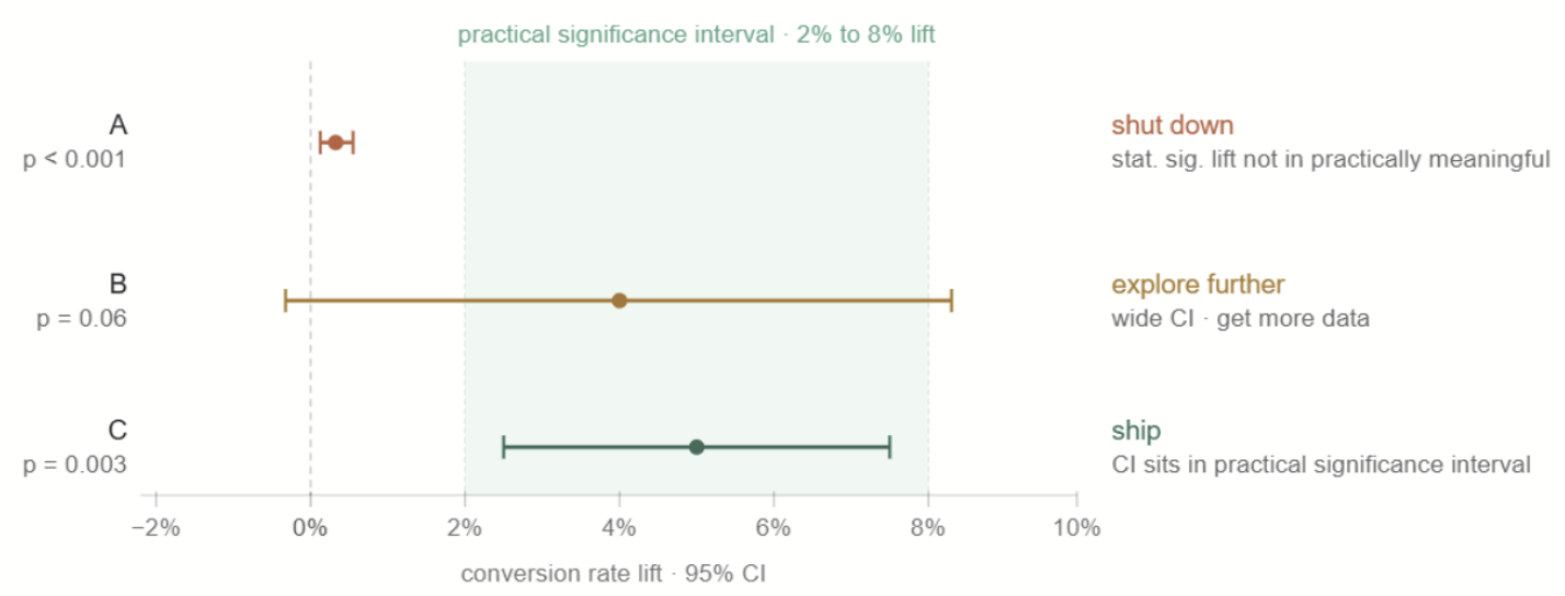
Image source: Optimizely
3. Learn from “non-significant” experiments
A “non-significant” p-value closes the statistical chapter but opens a behavioral one. Before concluding a variant had no effect, use your analytics tools to examine user behaviors. Funnel analysis can reveal whether the variant moved users through an intermediate step even if it failed to shift the final conversion metric. Session replays show whether and how users noticed or interacted with the changed element. Cohort analysis can identify effects confined to specific user segments diluted in aggregate data.
For example, an American online retailer tested if their new purchase experience was better than the old one and if it would boost conversion rates. But the experiment showed no significant difference in conversion rates between the new design and the old one. If they look closer by analyzing the purchase funnel step-by-step, they'll see that people in the new design group actually took longer to complete their purchases than those in the old design group, as the graph below shows. This might mean their new purchase experience isn’t as good as they expected.
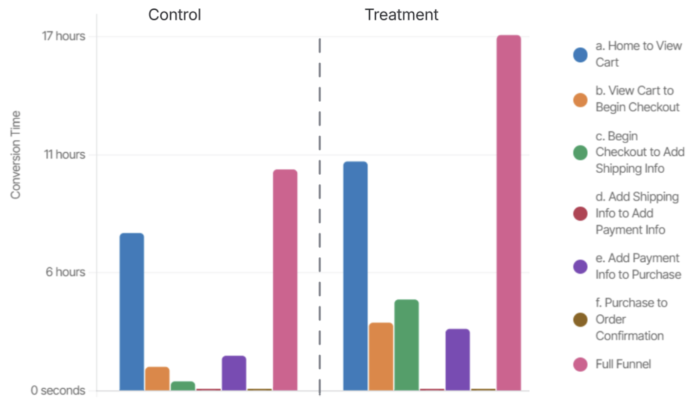
Image source: Optimizely
Also, if they look closer at the conversion time by visitors' browsers, they'll see that Chrome users in the treatment group spent a lot more time on the purchase process. This could mean there are some tech bugs in the code made for Chrome users. It might help to have the engineering team review the code.
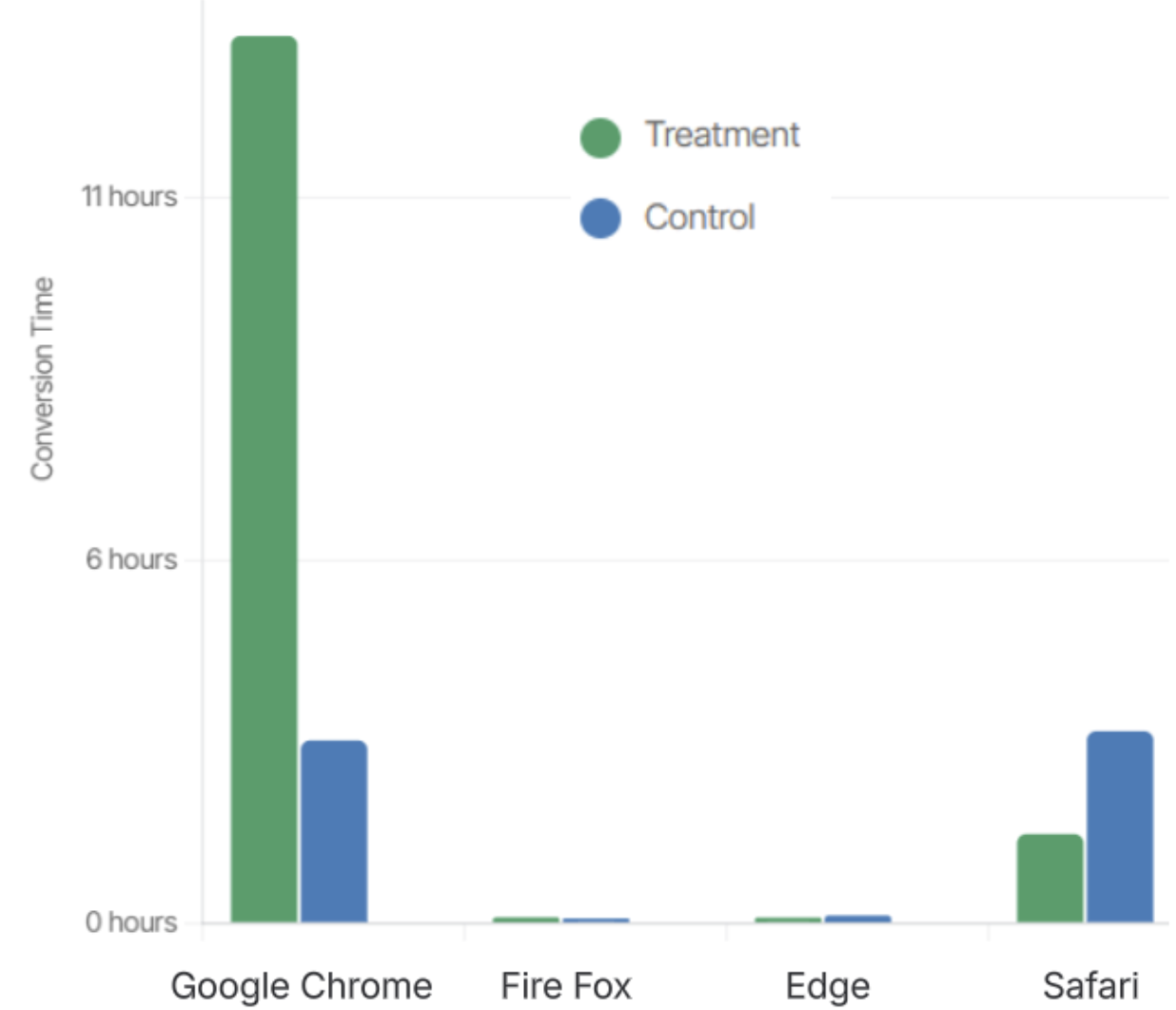
Image source: Optimizely
These exploratory follow-ups build your business's knowledge base and refine the hypothesis for the next experiment, which is how effective experimentation compounds over time.
---------------------------------------------------------------------------------------------------------
References
Biau, D.J., Jolles, B.M., & Porcher, R. (2010). P Value and the Theory of Hypothesis Testing: An Explanation for New Researchers. Clinical Orthopaedics and Related Research, 468, 885–892.
Fisher RA. (1956) Statistical methods and scientific inference.
Gelman, A., & Stern, H. (2006). The Difference Between "Significant" and "Not Significant" is Not Itself Statistically Significant. The American Statistician, 60, 328–331.
Greenland, S., Senn, S.J., Rothman, K.J., Carlin, J.B., Poole, C., Goodman, S.N., & Altman, D.G. (2016). Statistical tests, P values, confidence intervals, and power: a guide to misinterpretations. European Journal of Epidemiology, 31, 337–350.
Kennedy-Shaffer, L. (2019). Before p < 0.05 to Beyond p < 0.05: Using History to Contextualize p-Values and Significance Testing. The American Statistician, 73(S1), 82–90.
Wasserstein, R.L., Schirm, A.L., & Lazar, N.A. (2019). Moving to a World Beyond "p < 0.05." The American Statistician, 73(S1), 1–19.